ESM 263 Geographic Information Systems

Assignment 2 - Sea level rise in Santa Barbara

Due at Fri 2023-02-10 23:59

CONTENTS

• Assignment 2 - Sea level rise in Santa Barbara
  • Introduction
    • Tasks
    • Grading
    • Problem
    • Available data
  • Task 1 (optional): Tutorials
  • Task 2: Geospatial analysis and results data
    • Setup
    • Spatial join
    • Calculate flooded area
    • Calculate cumulative values
  • Task 3: Map results
  • Task 4: Turn in your work

Introduction

Tasks

1. Work through tutorials.
2. Perform a geospatial analysis using QGIS, and produce results data.
3. Design a map to communicate your results.
4. Submit your work to course website.

Grading

This assignment is worth 20 points: 10 points for your map and 10 points for your data, awarded according to the evaluation rubric. Your map must present your results accurately and clearly, and adhere to cartographic design principles. Your data must use correct units, data types, and file format.

Problem

In this homework, we’ll analyze some potential impacts of sea-level rise in the city of Santa Barbara, ranging from likely (~0.5 m) to catastrophic (~4 m; e.g., a continental ice sheet collapse). To reduce computational requirements, we’ve restricted our region of interest (ROI) to the downtown Santa Barbara area.

Your assignment is to estimate the cumulative impact of nine scenarios of sea level rise: 0 m, 0.5 m, 1.0 m, … , 4 m increases in mean sea level. You will compute three metrics for each sea level rise scenario, as shown in Table 1.

S sea level rise (meters)	A area flooded (hectares)	P parcels count	L flooded property losses ($millions)
0	?	?	?
0.5	?	?	?
1.0	?	?	?
1.5	?	?	?
2.0	?	?	?
2.5	?	?	?
3.0	?	?	?
3.5	?	?	?
4.0	?	?	?

Table 1: Results template

Again, the values of A, P, and L are cumulative: they apply to all areas affected by a corresponding amount of sea level rise (e.g., the values for a sea level rise of n meters should represent the total impact of a sea level rise from 0 to n meters.)

NOTE: The 0 m scenario will still show a few low-lying properties as flooded, so you must include it in your analysis.

Available data

The data you need are in HW2.gpkg (in HW2.zip). The following layers are provided:

• ROI: a rectangle defining the region-of-interest (ROI) for your analysis
• SLR_scenarios: polygonal features covering the areas inundated by each incremental sea level rise scenario
  • i.e., an SLR_m value of n means the feature covers the area inundated by a sea level rise from n to 0.5 + n meters.
  • The inundation features were generated from a high-resolution digital elevation model extracted from the NOAA’s 2009 - 2011 CA Coastal Conservancy Coastal Lidar Project dataset.
  • Only features selected by the ROI have been retained.
• parcels: Santa Barbara county assessor’s parcels
  • These polygonal features were extracted from the 07 March 2010 version of Tax Assessment Parcels (without Owner Names or Sales Data), obtained from the Santa Barbara County Enterprise Geographic Information System. Metadata was provided by Zacharias Hunt, Santa Barbara County Geographic Information Officer.
    • These data are no longer available online ☹️
  • The attributes of these features are described in ParcelMetadata.pdf (in HW2.zip).
  • Only features selected by the ROI have been retained.
• SB_city, SB_county, California: Layers containing outlines of the city and county of Santa Barbara and the state of California.
  • These layers aren’t necessary for your analysis, but may be useful in constructing your final map.

All data are in the NAD 83 / California Albers projection (EPSG:3310).

Task 1 (optional): Tutorials

Work through Lab 8: Spatial Selection of the Bolstad book.

NOTE: The Lab 8 instructs you to edit a table stored in a .csv file. Don’t do this—editing .csv tables in QGIS is buggy. Instead, export the table into a geopackage, remove the .csv from your map, then add and edit the geopackage version.

Task 2: Geospatial analysis and results data

Setup

Download HW2.zip and extract the contents into your ESM263 folder.

Create a new map in QGIS called HW2.qgz and add all the layers ROI, parcels, and SLR_scenarios.

Read the metadata in ParcelMetadata.pdf. There are several property value attributes. We will use NET_AV: the net assessed value (in USD) for the parcel.

Spatial join

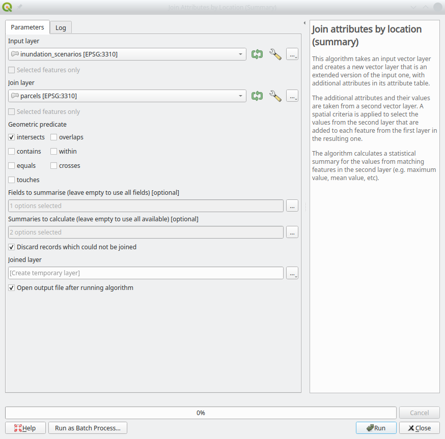
You’ll perform a spatial join of the parcels and the SLR_scenarios layers. Use the Join attributes by location (summary) tool.

NOTE: There is also a Join attributes by location tool. Make sure to use the one whose name ends with “(summary)”

• Set Input layer to SLR_scenarios.
• Set join layer to parcels.
• For Geometric predicate, check intersects (the default).
• Set Fields to summarise to NET_AV.
• Set Summaries to calculate to sum and count.
• Check Discard records which could not be joined.

A tip to help you select the correct input and join layers: The input layer is the one that will be modified with new attributes in the spatial join. Since we want the sum of the parcel values and the count of the parcels to be added to the inundation scenarios, it will be the input layer.

Figure 3: Spatial Join

Rename the newly created (temporary) layer to results and save it into a new geopackage.

Calculate flooded area

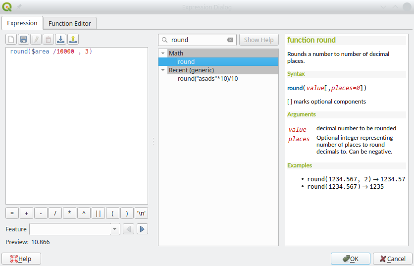
If you did everything correctly, the results layer’s attribute table contains the correct values of the count of the inundated parcels and their total assessed value. However, you’re missing the flooded area. Use the field calculator to create a new field flooded_area (don’t just call it area; that will cause errors when you try to save the layer to a geopackage.)

• Coordinates in the California Albers projection are in meters; thus, calculated areas will be in units of square meters, which you need to convert to hectares.
• Use the round() function to round your the calculated area a reasonable number of significant digits.

Figure 4: Use field calculator to calculate the area

Calculate cumulative values

You now have the following attributes for each 0.5 increment of sea level rise represented by the features in SLR_scenarios:

• NET_AV_count: number of parcels flooded
• NET_AV_sum: value of those flooded parcels ($ USD)
• flooded_area: area flooded (hectares)

However, you will recall that what you really want are cumulative values—e.g., to get the total number of parcels flooded by n meters of sea level rise, you’ll need to sum up the number of parcels flooded by all sea level rise increment less than or equal to n.

Sounds like a job for Excel, right? Well, it turns out that it’s not too difficult (if not exactly obvious how) to do this in QGIS. Just like we calculated the flooded area using a Field Calculator expression, we can use a slightly more complicated one to do the cumulative sums—here it is so you can copy-n-paste it:

with_variable(
    'SLR_m',
    SLR_m,
    sum(flooded_area, filter := SLR_m <= @SLR_m)
)

Change flooded_area to NET_AV_count or NET_AV_sum to calculate the cumulative values for those columns. (Remember to convert NET_AV_sum to $millions).

Name the new columns A, P, and L (of course…).

Task 3: Map results

Design a map that communicates your results, including a table with the relevant fields of the attribute table of your results layer. Consider these questions:

• What are the data source(s) and units for your results?
• Which information from your results do you want to communicate?
• What is an appropriate symbology to communicate your results visually?
• How will you layout and organize your map elements?
• How will you describe your results in these map elements?
• How will you design your base layers to provide appropriate context for your results?

Task 4: Turn in your work

1. Export your map as a PDF document to HW2.pdf using the same settings as in Assignment 1.
2. Export your results layer’s attribute table to a CSV file named HW2.csv. Make sure that the CSV file only has the 4 fields SLR_m, A, P, and L.
3. Rename your files to include your full name, and use correct capitalization with no spaces or punctuation; e.g., HW2MortimerSnerd, NOT HW2-mortimer-snerd or hw2mortimersnerd:
   • HW2.pdf to HW2FirstLastName.pdf
   • HW2.csv to HW2FirstLastName.csv
4. Verify that your PDF document displays correctly, and that your CSV file is readable by QGIS (and/or Excel) and has the correct field names and data types.
5. Upload your PDF and CSV files to the Assignment 2 link on Canvas.